PyTorch 操作

训练

model.train() # set to train mode
optimizer = torch.optim.SGD(model.parameters(), lr = 1e-5, momentum = 0.9)
criterion = torch.nn.MSELoss(reduction = "mean") # set loss function
train_pbar = tqdm(train_loader, position = 0, leave = True)

for x, y in train_pbar:
    x, y = x.to('cuda'), y.to('cuda') # move data to GPU
    pred = model(x)                   # output predict result
    loss = criterion(pred, y)         # calc loss
    loss.backward()                   # calc gradient
    optimizer.step()                  # update parameters
    optimizer.zero_grad()             # clear gradient

测试

model.eval() # set to eval mode
train_pbar = tqdm(train_loader, position = 0, leave = True)

for x, y in train_pbar:
    x, y = x.to('cuda'), y.to('cuda') # move data to GPU
    with torch.no_grad():             # disable gradient calc
        pred = model(x)               # output predict result
        loss = criterion(pred, y)     # calc loss
	total_loss += loss.cpu().item() * len(x)

Deep Learning（深度学习）

步骤

1. Define a set of function
2. Goodness of function
3. Pick the best function

Backpropagation（反向传播）

Forward Pass

$$\frac{\partial z}{\partial w} = \texttt{last neuron output}$$

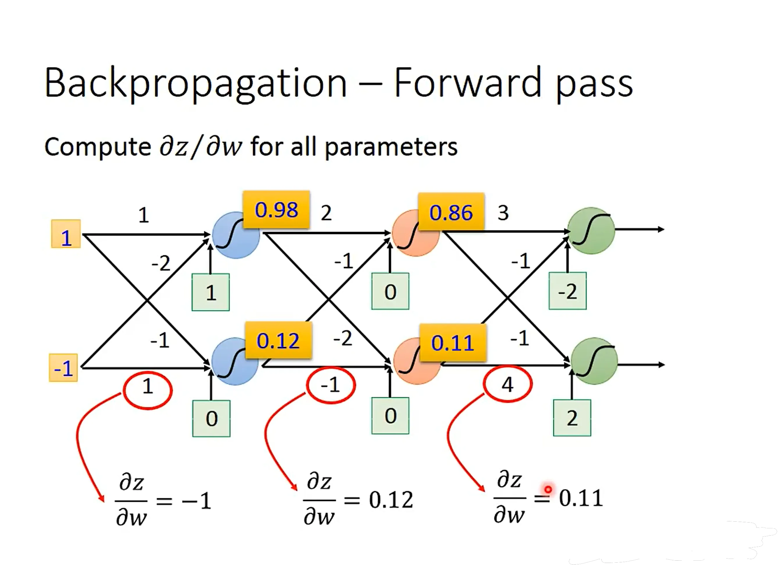
当前偏微分等于上一级神经网络的输出。

Backward Pass

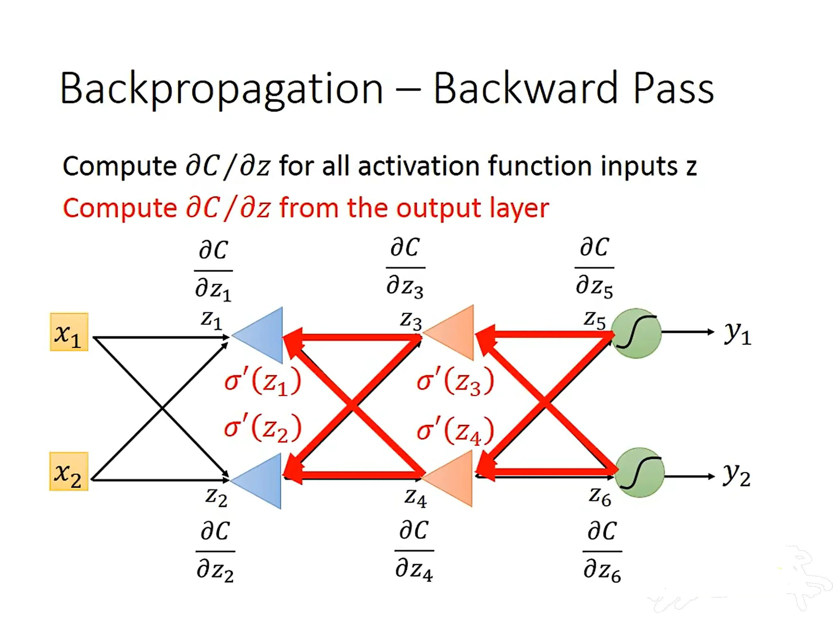
反向建立神经网络，就可以通过输出直接得到偏微分。

预测训练过程

Design the model

可以设计多元函数，但是过于复杂的函数往往会导致函数 过拟合。

Regularization

$$L = \sum_n[{\hat y}^n-(b+\sum{w_ix_i})]^2+\lambda\sum w_i^2$$

添加对 $w$ 的限制，使得生成的函数有平滑性要求。

分类训练过程

Design the model

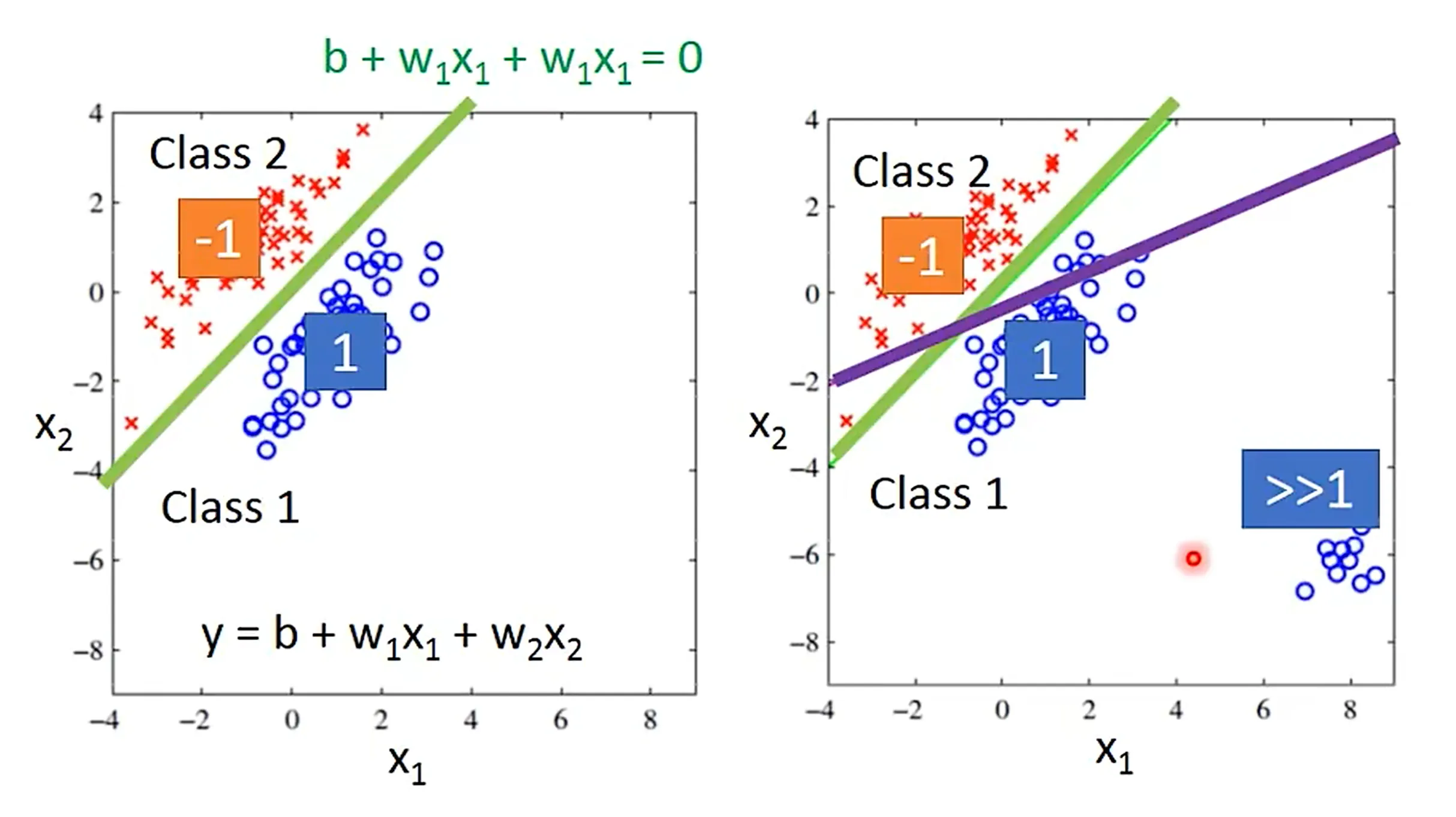
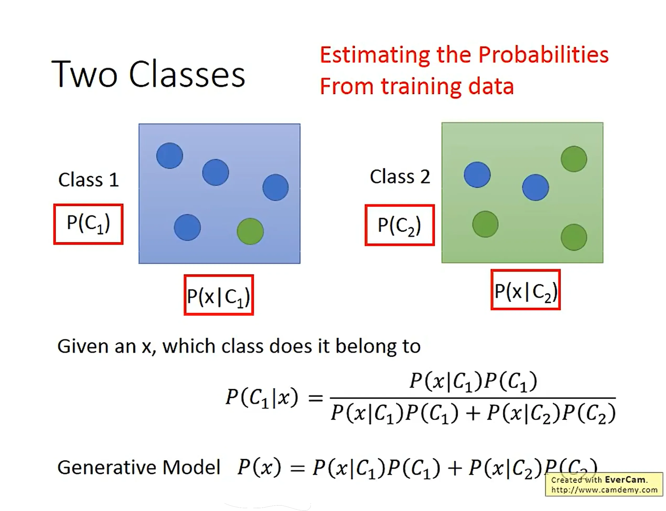
直接使用多元函数拟合会导致函数偏移，分类时候使用贝叶斯。

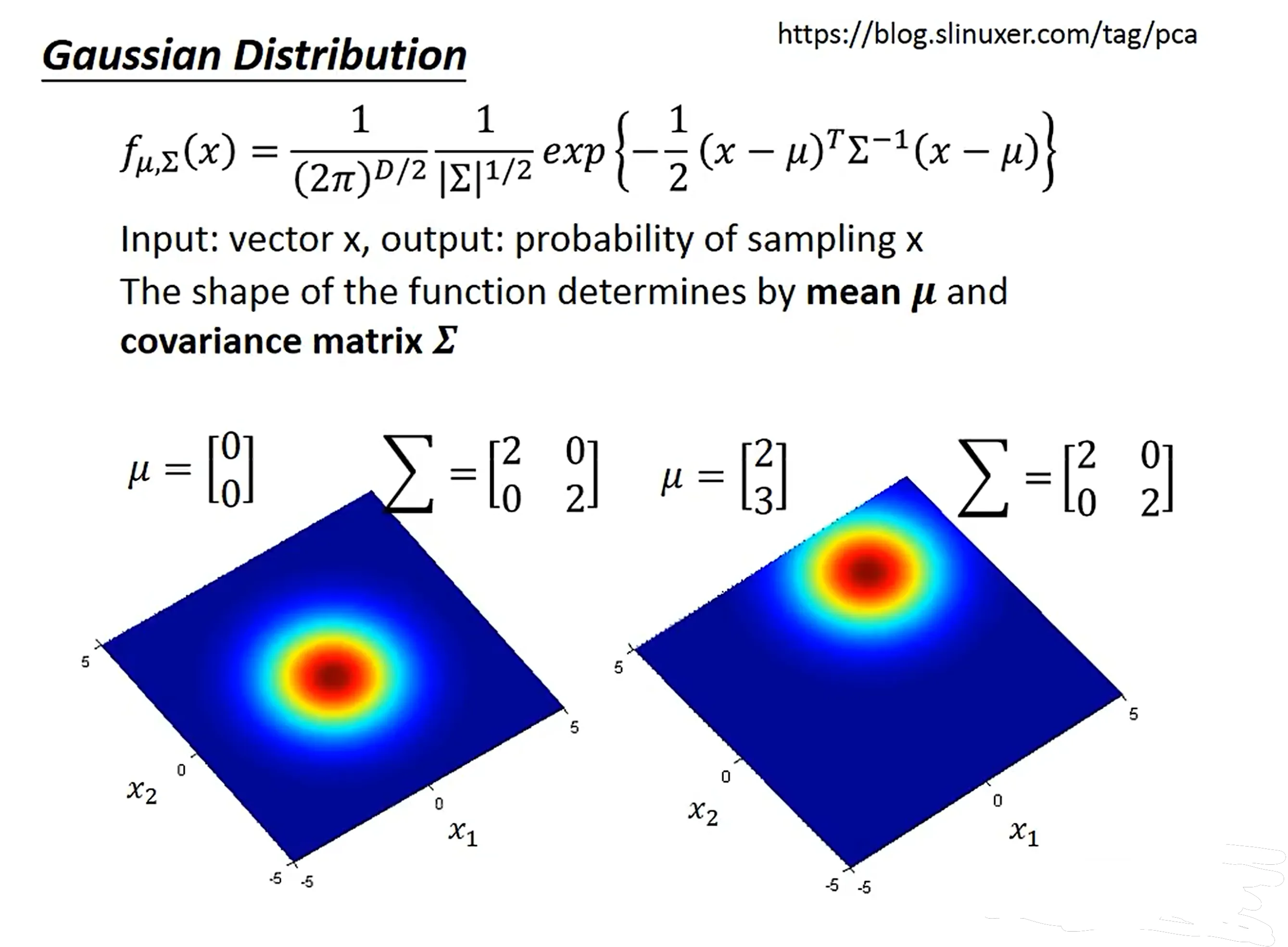
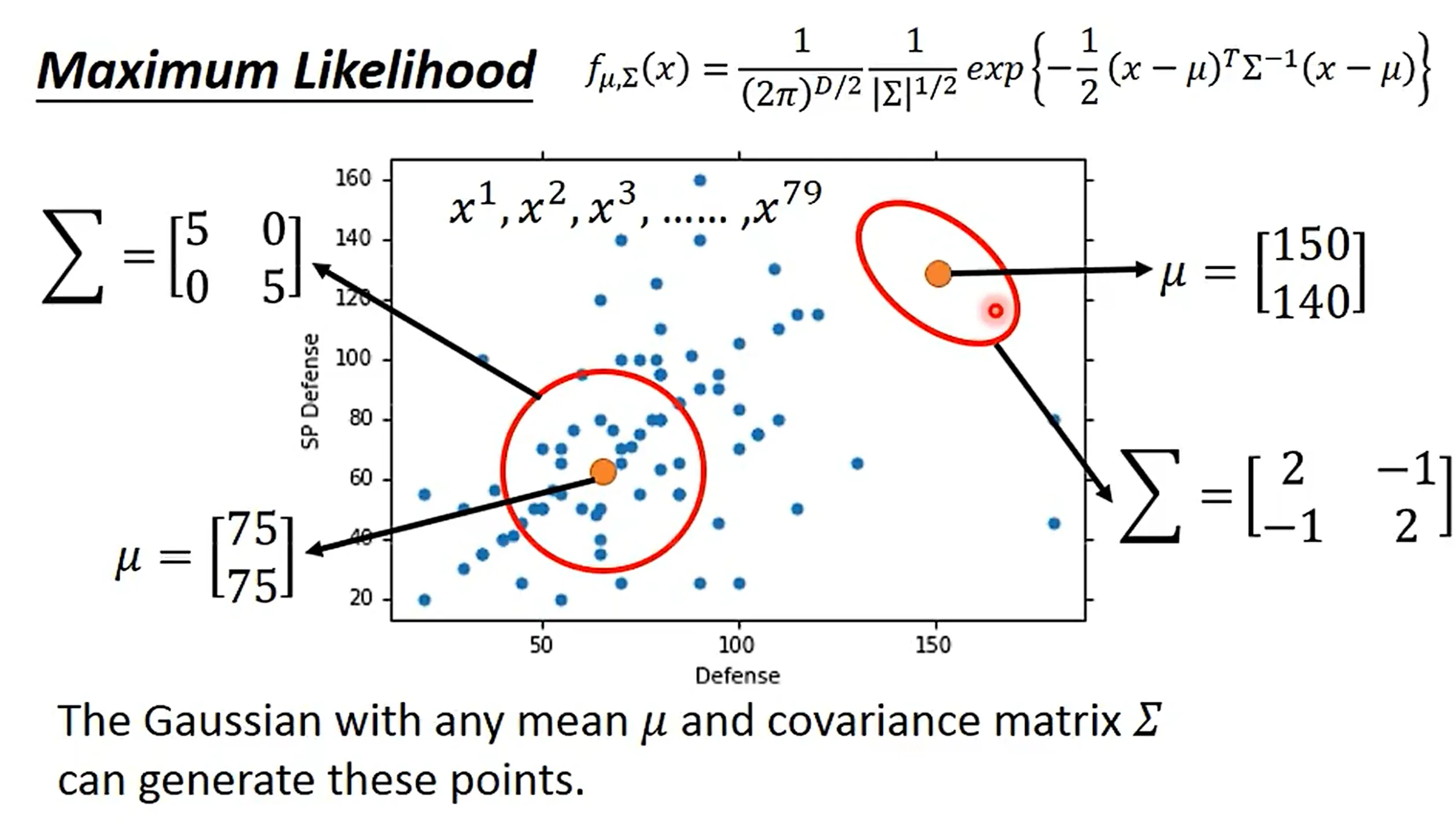
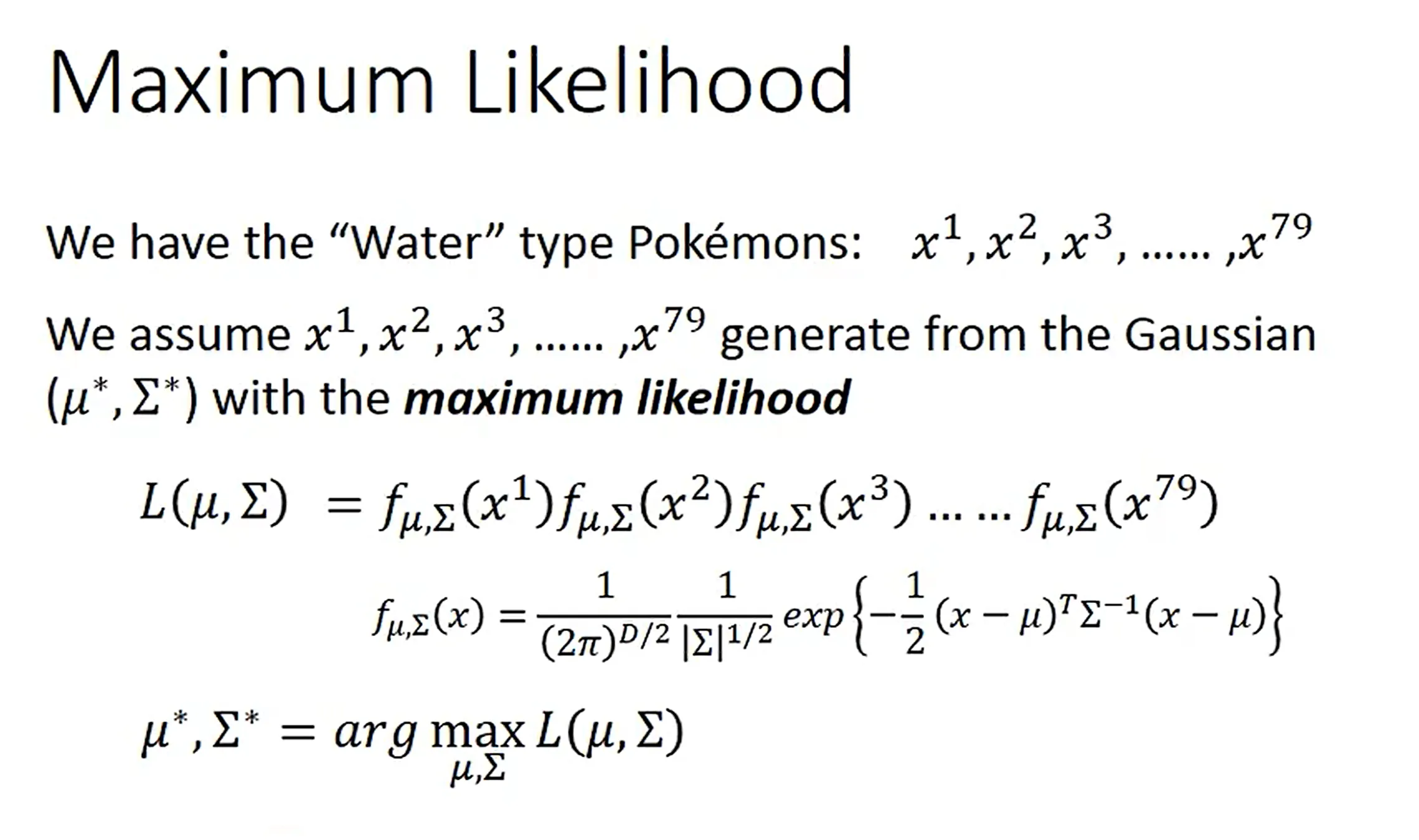
使用高斯函数可以估计邻近点的概率。通过不断修改 $\mu$ 和 $\sigma$ 使得高斯函数逐渐逼近。

$$P(C_1|x)=\frac{P(x|C_1)P(C_1)}{P(x|C_1)P(C_1)+P(x|C_2)P(C_2)}$$

如果结果超过一半，则可以分到第一类。

f(x) = \left{ \begin{array}{lr} g(x)>0 & \Rightarrow \texttt{Output = class 1} \ else & \Rightarrow \texttt{Output = class 2} \ \end{array} \right.

$$L(f)=\sum_n\delta(f(x^n)\ne\hat y^n)$$

逻辑回归训练过程

Design the model

$$P_{w,b}(C_1|x)=\sigma(z)$$

$$z=w\cdot x+b=\sum_i{w_i\cdot x_i}+b$$

$$f_{w,b}(x)=P_{w,b}(C_1|x)$$

修改 $w$ 和 $b$ 可以得到一系列函数。

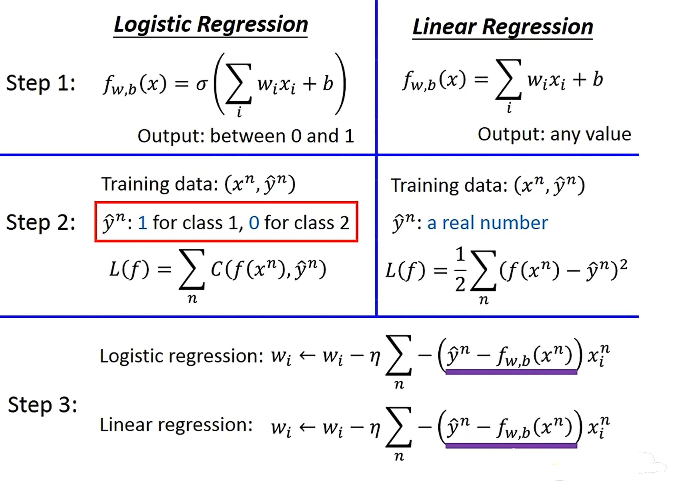
Choose Loss Function

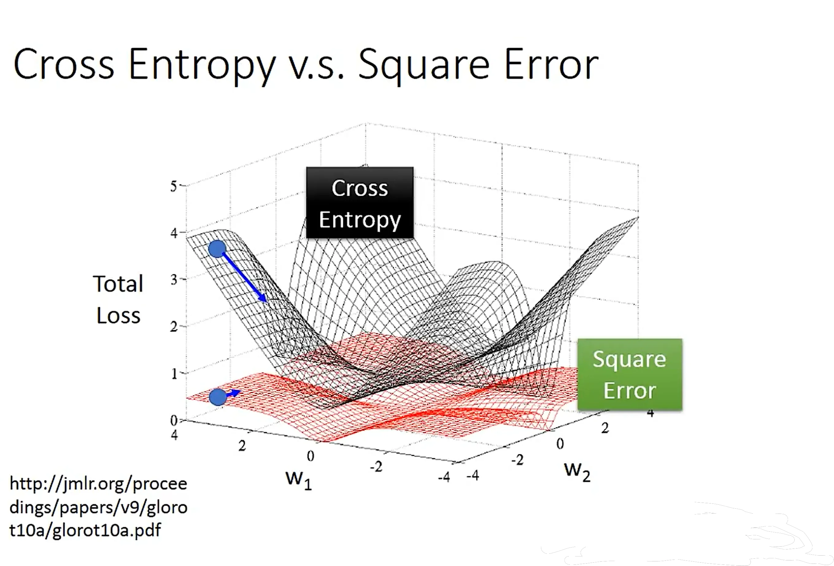
Cross Entropy 可以有更快的收敛速度。

Multi-class Classification

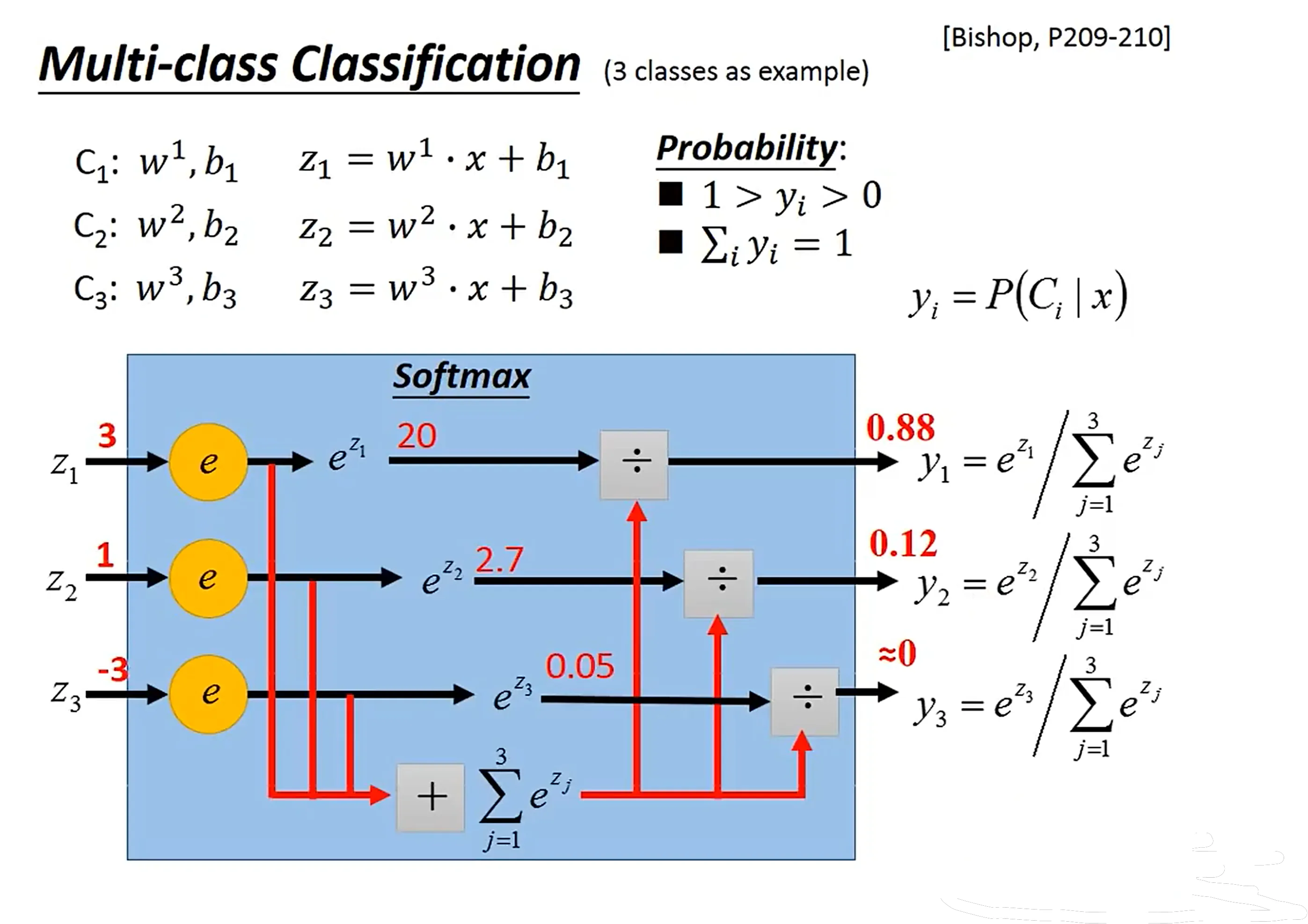
逻辑回归的缺陷

有时候无法完全分离两类，需要使用深度神经网络来实现。